Log transformation has been one of the commonly, if not the most popular, used transformations in analyzing gene expression data. While zero counts is fairly prevalent in many gene expression data, e.g. scRNA-seq data, log transforming zero counts encounters a numeric issue, providing negative infinity as a result. To address it, pseudocounts, a small, arbitrary positive number \(p\) (e.g. \(p=1\)), is added to the gene expression data before taking the log transformation. There are many literature documenting the practice of log-transformation with pseudocounts (for simplicity, we’ll refer it to as log-transformation unless noted otherwise) could distort the estimation marginal mean (Booeshaghi and Pachter 2021; Lun 2018; Townes et al. 2019). Few has explored how the pseudocounts would mathematically distorts the fold change even with accurate estimation of marginal mean.
What is fold change?
It is well believed that the gene expression data we measure represents relative abundance of gene. Hence, comparing to modeling the absolute differences (the subtraction between to number), most people argues it would be more appropriate to measure the changes of gene expression as an ratio, commonly referred to as fold change or equivalently the log fold change. For example, if you have two numbers representing the relative abundances of a gene in two samples \(A\) and \(B\), \(\mu_A\) and \(\mu_B\), the fold change between the two samples is the division of the two number \(\mu_A/\mu_B\) and the log fold change \(\log(\mu_A/\mu_B) = \log(\mu_A) - \log(\mu_B)\). It is very common to report log fold change instead of log fold changes, because log fold change converts the statistics on the multiplicative scale to the additive scale, and providing a convenient modeling choice, general linear models.
While the author want to emphasizing log transformation is extremely confusing due to the ambiguous nomenclature and notation of logarithms with different bases, the confusion doesn’t change the assessment in this article up to a constant scaling factor \(c\), \[
\log_a(x) = \ln(x)/c \quad \text{where } c=\ln(a)
\]
Fixed Reference
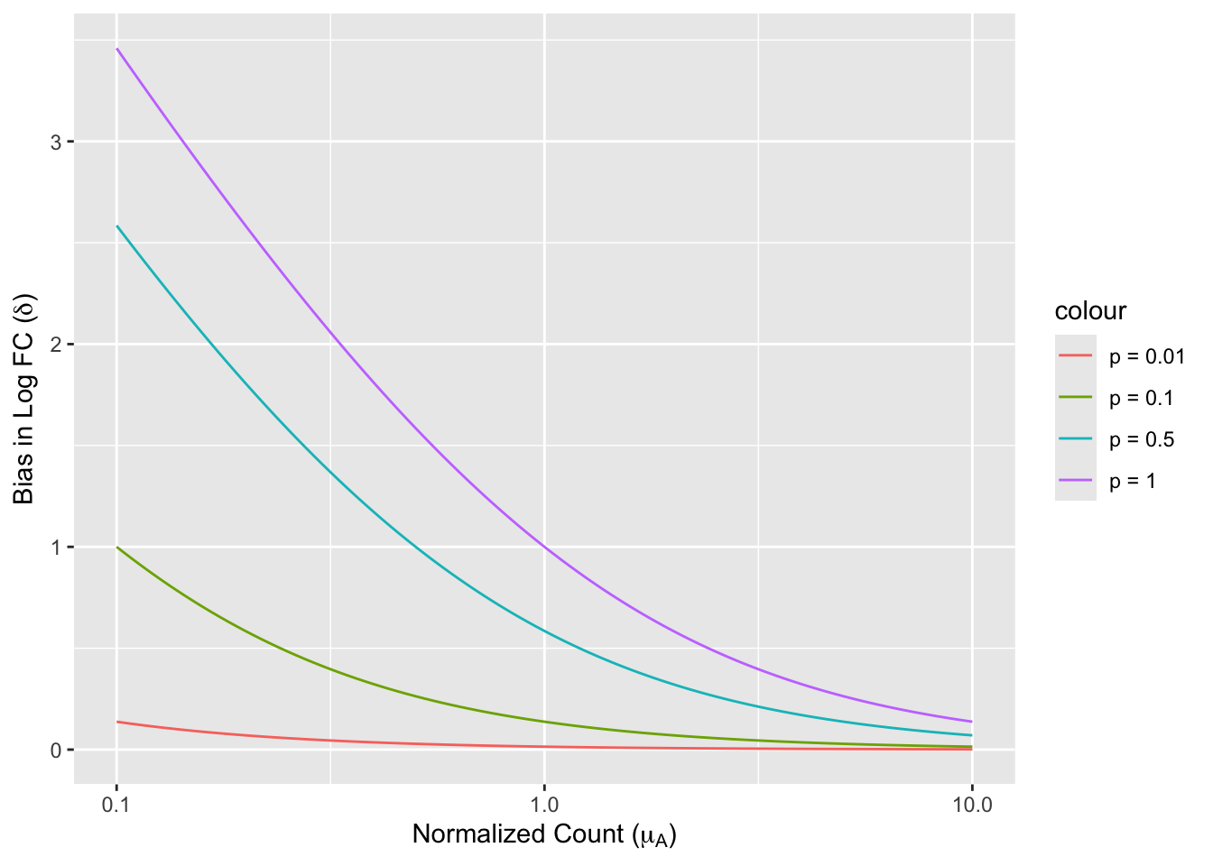
We first consider the distortion that pseudocounts causes in the simpliest setting, fixing a reference level, i.e. the denominator. A real-world appication is similar to a Student’s t-test with the hypothesis \(\mu_A = \mu\), where \(\mu\) is an known constant.
Without Pseudocounts
With Pseudocounts
data
\(\log(\mu_A)\)
\(\log(\mu_A+p)\)
log fold change
\(\log(\mu_A) - log(\mu)\)
\(\log(\mu_A+p) - log(\mu)\)
The discrepency between the two quantities is the bias that pseudocounts introduces. \[\begin{align*}
\delta &= (\log(\mu_A+p) - log(\mu)) - (\log(\mu_A) - log(\mu))\\
& = \log(\mu_A+p) - \log(\mu_A) = (\log 1+\frac{p}{\mu_A}).
\end{align*}\]
Similar, we can consider a more challenging setting where we don’t have a fixed reference level, which mimics the two-sample t-test setting.
Without Pseudocounts
With Pseudocounts
data
\(\log(\mu_A), \log(\mu_B)\)
\(\log(\mu_A+p), \log(\mu_B+p)\)
log fold change
\(\log(\mu_A) - log(\mu_B)\)
\(\log(\mu_A+p) - log(\mu_B+p)\)
The discrepency between the two quantities is the bias that pseudocounts introduces. \[\begin{align*}
\delta &= (\log(\mu_A+p) - log(\mu_B+p)) - (\log(\mu_A) - log(\mu_B))\\
& = \log\frac{\mu_B(\mu_A+p)}{\mu_A(\mu_B+p)} = \log\frac{\mu_A\mu_B+p\mu_B}{\mu_A\mu_B+p\mu_A}\\
& = \log\frac{1+p/\mu_A}{1+p/\mu_B} = \log (1+\frac{p\mu_B - p\mu_A}{\mu_A\mu_B + p\mu_A}).
\end{align*}\]
library(plotly)x <- y <-seq(0.1, 10, by =0.1)two_fun <-function(x, y, p)function(x,y) outer(x, y, FUN =function(x, y) log2((1+p/x)/(1+p/y)))z_1 <-two_fun(x, y, p=1)z_0.1<-two_fun(x, y, p=0.1)plot_ly(x =~x, y =~y) |>add_surface(z =~z_1(x,y)) |># add_surface(z = ~z_0.1(x,y), opacity = 0.5)layout(title ="p=1",scene =list(xaxis =list(title ="Normalized Count \\mu_A"),yaxis =list(title ="Normalized Count \\mu_B"),zaxis =list(title ="Bias in Log FC (\\delta)") ) )
Note: The one-group setting is different from the two group_setting, in the sense if you add 1 to the reference level…
Regression Setting
In the previous two examples, the reference level, i.e. the dividend in the division, is (fairly) clear. However, if we extend the problem to the regression setting, including the two-group testing scenario as an example, the reference level is less obvious.
For example, if we think the pseudotime analysis as an example of the regression setting, we are interested in regressing the gene expression, \(X\), as a function of time, \(T \in \{t_0, t_1, \dots, t_n\}\). To simplify, we assume the function of time is linear with the gene expression \[
Y = \beta_0 + \beta_1T + \epsilon.
\] To naively interpret the model, \(\beta_1\) is the log fold change per one-unit change in time, and \(\beta_0\) is the log-transformed gene expression at some reference time point (\(t_0\)), e.g. \(t_0 = 0\). Here, we are interested in measuring how the change in \(\beta_1\) with and without adding pseudo-count.
# Sim log_y without errorpseudo_t <-seq(0, 3, by =0.1)beta_0 <-0.5; beta_1 <-1log_y <- beta_0 + beta_1*pseudo_t# Sim log_y plus 1y <-2^(log_y)log_y1p <-log2(y+1)# Pltggplot() +geom_point(aes(x = pseudo_t, y = log_y,group ="log_y", color ="log_y") ) +geom_point(aes(x = pseudo_t, y = log_y1p,group ="log_y1p", color ="log_y1p") )
ggpubr::ggarrange(ggplot(newdat) +geom_point(aes(x = x, y=y, color = clus_log2_z)),ggplot(newdat) +geom_point(aes(x = x, y=y, color = clus_log1p)) )
Why this is important?
Limitation of this report
Does the bias \(\delta\) matter much? I didn’t look at the percentage of bias to the true effect size, i.e. \(\delta/\log\text{FC}\) where \(\log \text{FC} = \log(\mu_A) - \log(\mu_B)\).
This problem is not scientifically interesting if the percentage of bias is small.
The simulation study of spatial modeling lacks of repetition to account for randomness in clustering results, i.e. the initial data points.
The spatial effect might be too aggressive in the example.
For nonlinear effect estimation, the model fitting is slightly more complicated, and could behave differently. (probably not much).
References
Booeshaghi, A Sina, and Lior Pachter. 2021. “Normalization of Single-Cell RNA-Seq Counts by Log (x+ 1) or Log (1+ x).”Bioinformatics 37 (15): 2223–24.
Lun, Aaron. 2018. “Overcoming Systematic Errors Caused by Log-Transformation of Normalized Single-Cell RNA Sequencing Data.”BioRxiv, 404962.
Townes, F William, Stephanie C Hicks, Martin J Aryee, and Rafael A Irizarry. 2019. “Feature Selection and Dimension Reduction for Single-Cell RNA-Seq Based on a Multinomial Model.”Genome Biology 20: 1–16.